How CP-SAT Reasons: The Search Core
CP-SAT is easy to use as a black box: you declare variables and constraints, call solve, and read off an answer, often without knowing what the engine did in between. That is usually enough. But when a model is unexpectedly slow, a log line resists interpretation, or a small reformulation changes everything, there is nothing underneath to reason about. This text is for the reader who already builds CP-SAT models and now wants to understand how the solver reasons, both to model more deliberately and out of curiosity about the machinery.
Google OR-Tools’ CP-SAT behaves at once like a constraint-programming solver, a SAT solver, and a mixed-integer programming solver, and it is not obvious how one engine manages to be all three. At heart the search is a simple loop: propagate to rule out values that cannot work, branch by making a guess when propagation stalls, and learn from each dead end so the same mistake is not repeated. The idea that ties this loop together is lazy clause generation. A CDCL learning core reasons over integer bounds rather than plain Booleans; constraint propagators and a linear relaxation feed it deductions it can record and reuse. A variable is a pair of bounds, every propagation carries a reason for why it fired, and each dead end is distilled into a learned clause that lets the search backjump past the choices that were never to blame. Around this core sit the accelerators that make it fast in practice: a lazy Boolean encoding that materializes only the literals the search actually touches, a dual-simplex LP relaxation that supplies bounds and cutting planes, restarts that reshape the search tree, and a parallel portfolio of complementary strategies that share what they learn. Seeing how these parts interlock is what turns the solver from a black box into a machine you can reason about.
 This is an in-depth companion chapter. It is also available as a typeset PDF with full typography, and its content is generated from that LaTeX source. |
1 What kind of solver is CP-SAT?
CP-SAT solves constraint optimization problems over integer variables. You declare integer and Boolean variables with finite domains, post constraints that link them, and optionally add a linear objective. The solver then finds an assignment that satisfies every constraint and optimizes the objective, or proves that none exists. That is the complete-search promise. Under a time or resource limit, CP-SAT may instead return the best solution and bound it has found so far, or report that the status is still unknown.
There are other solvers with that promise, but what makes CP-SAT distinctive is its lineage. It fuses two solver traditions that historically lived apart:
- Constraint Programming (CP), whose strength is propagation: rich, problem-specific reasoning that prunes domains (“if these three tasks cannot overlap and two are already scheduled here, the third cannot start before time 12”). Figure 1 shows the idea on a Sudoku.
- Conflict-Driven Clause Learning (CDCL) SAT, whose strength is learning from failure: whenever search reaches a dead end, it distills the failure into a reusable rule, a “nogood,” so that it never repeats the same mistake (Figure 2).
A one-line example shows what propagation means. Suppose two variables \( x, y \in \{0,1,\dots,5\} \) are tied by the constraint \( x + y \le 5 \), and the search guesses \( x \ge 4 \). The constraint immediately forces \( y \le 1 \), so the solver shrinks \( y \)’s domain to \( \{0,1\} \) with no further guessing. That shrinking is propagation: a constraint ruling out the values a variable can no longer take. The piece of code that does it for one constraint is its propagator. Figure 1 shows the same mechanism at Sudoku scale, where one forced value cascades into many.
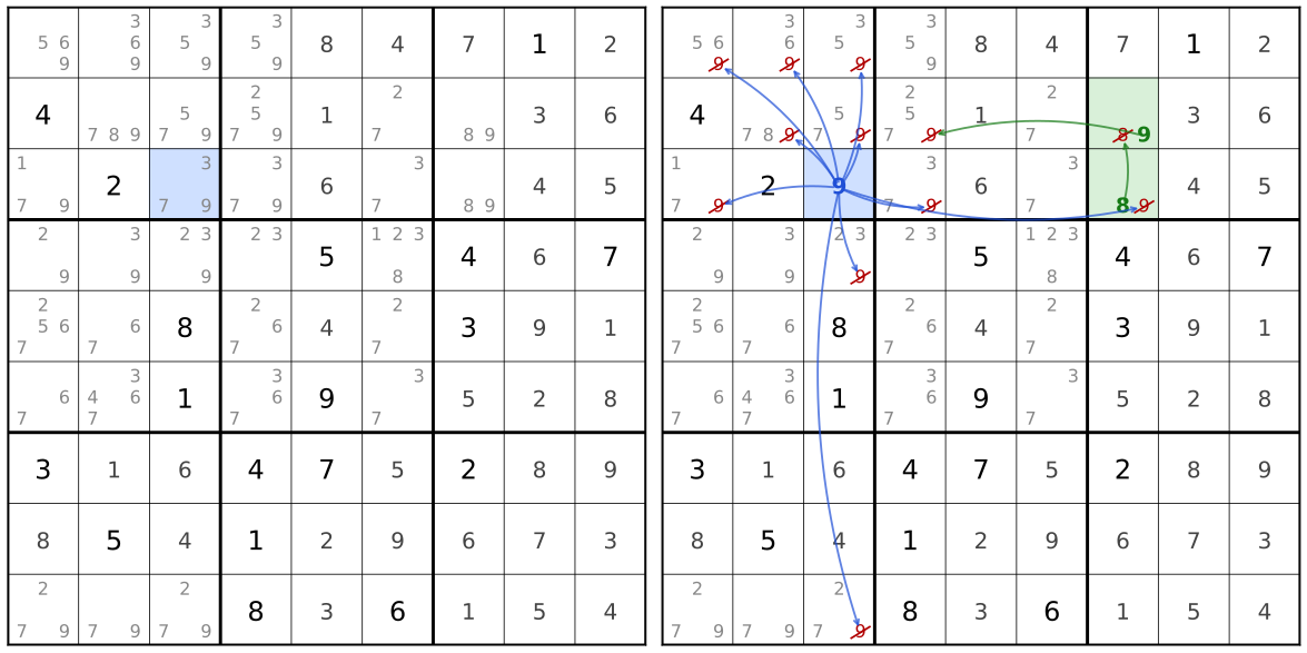
Figure 1. Propagation on a Sudoku: each cell is a variable, the all-different constraints on rows, columns, and boxes are the propagators, and the small pencil marks are each cell’s remaining candidates. Left: the givens propagated as far as they go; every empty cell still has several candidates and none is forced, so search must guess. Right: we guess a blue value; the propagators strike it from every peer (blue arrows), one peer loses its last alternative and is forced, which forces a green value, and the deductions cascade to a new fixed point with no further guessing.
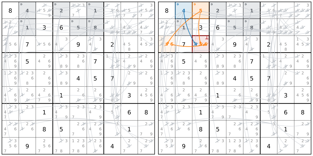
Figure 2. Conflict analysis on a Sudoku. Left: six guesses (grey, tagged \( D \)) have been placed and propagated, and nothing has failed yet. Right: a seventh guess (orange) propagates and empties one cell’s domain (red, \( \bot \)): a conflict. Tracing the struck candidates backward shows that only two of the seven guesses are jointly to blame (the orange one and a blue one); the other five never touched this cell. From these two the solver learns a SAT clause (a nogood) that bars the combination forever, then backjumps past the five irrelevant guesses instead of just undoing the last one.
Classic CP search is good at pruning but tends to be amnesiac: it backtracks and forgets why it failed. Classic SAT learns effectively but only speaks in Boolean clauses and cannot compactly express arithmetic relations among integer variables. CP-SAT’s central idea, lazy clause generation, combines the two: CP-style propagators perform the pruning, but every pruning step is justified by a reason from which the CDCL engine can learn. The result is a CP solver with a SAT solver’s memory.
 Background The developers trace CP-SAT’s lineage directly to the lazy-clause-generation work of the late 2000s, notably Peter Stuckey’s pointed “search is dead” framing, and built CP-SAT by deliberately discarding the classic CP search machinery in favor of a learning SAT core. For a general introduction to the technique itself, see Krunal Patel’s “What is Lazy Clause Generation?” [1]; for the fuller story, see Stuckey’s talk on lazy clause generation [2] and the CP-SAT developers’ own overview talks [3, 4, 5]. |
Two further ingredients complete the picture. The rest of this text treats them as accelerators bolted onto the core (Section 6, Going faster), but they are central to what CP-SAT is, and any honest description should name them up front.
- A linear-programming relaxation, run as a propagator. Alongside the search, LP-enabled CP-SAT workers maintain a continuous LP relaxation of the model and re-solve it with the dual simplex as a high-cost propagator, typically after cheaper propagation has stalled. The LP relaxation feeds back global numeric bounds, reduced-cost reasoning, and cutting planes (Sections 6.1 and 6.2). This creates the bridge to the MIP (mixed-integer programming) world of branch-and-cut: a third solver tradition folded in beside CP and SAT, and the reason CP-SAT holds its own on problems with strong linear structure where pure propagation is weak.
- A parallel portfolio, not a single search. Given several threads, CP-SAT does not partition one tree. It runs a portfolio of workers instead, most of them differently configured copies of the same core (some LP-heavy, some pure CP/SAT, some core-guided on the objective), together with a set of primal heuristics. These workers attack the whole problem at once and continuously share the clauses and bounds they learn (Section 6.4).
So the compact answer to “what is CP-SAT?” is: a CDCL learning core, fed by CP propagation and an LP relaxation, diversified across a cooperating portfolio.
2 Foundations
This section assembles the search core from its parts: the data model every other piece reads and writes, the propagation that reasons over it, and the branching that turns a pruned domain into a concrete solution. We start with how a variable is stored, look inside a single propagator, sort out which high-level constraints are expanded away versus kept as propagators, and finish with how search drives a range down to one value.
|
Background A working familiarity with CDCL SAT solving (decisions, unit propagation, conflict analysis, clause learning, and backjumping) is not strictly required here, but it is highly recommended. CP-SAT layers a good deal on top of a CDCL core, so having seen how a plain CDCL solver works makes the rest considerably easier to follow. Readers who want that background first can start with Smock’s gentle visual introduction [6] (about 35 minutes), move on to Nadel’s more technical talk linking CDCL to optimization [7], and turn to Biere’s in-depth tutorial [8] (about four and a half hours) for the full machinery. Knuth’s fascicle [9] is the canonical written reference, useful either in place of the videos or alongside them. |
2.1 The data model: variables as bounds
Everything that follows rests on a single design decision: how the solver represents an integer variable while it is running. Once this idea is clear, the rest of the architecture (propagation, reasons, and learning) falls into place almost inevitably.
Variables are bounds, not values. An integer variable \( x \) with domain \( [0,10] \) is not stored as a tentative value, such as “\( x \) is currently \( 3 \).” It carries no working assignment at all: nothing like the fractional value a MIP branch-and-bound node rounds, or the running guess a heuristic nudges toward feasibility. Instead it is stored as a pair of current bounds, a lower bound \( \text{lb}(x) \) and an upper bound \( \text{ub}(x) \). Search and propagation never assign \( x \); they only narrow the gap between these two numbers, and \( x \) is fixed only once they meet.
This puts CP-SAT close to a classical finite-domain solver, which also narrows rather than assigns, but with one decisive difference. A finite-domain solver keeps the full set of surviving candidate values and lets a propagator strike any one of them, every even number say, out of the interior of a domain. CP-SAT’s propagators move only the lower and upper bounds. The integer trail reasons about \( x \) through those two numbers alone, treating the live domain as the interval \( [\text{lb}(x), \text{ub}(x)] \) between them. When the declared domain has holes, this interval is an over-approximation: bound propagation works on the enclosing interval, while the holes themselves are tracked separately, by presolve canonicalization and the integer encoding of Section 4.1. Until that section, treat every domain as a plain interval.
As the solver descends the search tree, the bounds tighten (\( \text{lb} \) rises and \( \text{ub} \) falls); when it backtracks, they relax again. Domains therefore shrink from the outside in and grow back the same way.
Two properties of this representation make it work:
- Monotonicity. Within one root-to-node path, the bounds only move inward. A propagator never has to reconcile competing updates; it only reads the tightest bounds known so far.
- Reversibility. Because a bound is a single number stamped with the decision level that set it, undoing work on backtrack is simple: pop every bound change made above the level to which the solver jumps. This integer trail, a stack of bound changes, is the same one that powers conflict analysis (Section 3.1).
The atomic fact: a bound literal. If variables are bounds, then the elementary statements the solver asserts and reasons about are bound literals: claims of the form
\[ [\![x \ge 5]\!] \qquad\text{or}\qquad [\![x \le 3]\!] . \]
The double brackets mark the claim as an object the solver holds, enqueues, and gathers into reasons, as opposed to the bare arithmetic relation \( x \ge 5 \); we write them where that literal-as-object reading is what matters and drop them in running prose where it is not. A bound literal is the integer analog of a Boolean SAT literal, and, crucially, it behaves like one in the two ways the learning machinery needs. (These are exactly what the source calls an IntegerLiteral; this text says “bound literal” throughout, but the two names refer to the same object.) It negates cleanly: over the integers, the negation of \( x \ge 5 \) is exactly \( x \le 4 \). Moreover, a conjunction of bound literals describes an interval, so the current domain \( [\text{lb},\text{ub}] \) is just the two literals \( x \ge \text{lb} \) and \( x \le \text{ub} \) held true at once. A variable is fixed when its bounds meet, \( \text{lb}(x) = \text{ub}(x) \): the interval has collapsed to a single value, and this is the only sense in which \( x \) ever “has” a value during search.
Why this unifies the whole solver. This representation lets a single engine reason about a Boolean variable with domain \( \{0,1\} \) and a wide integer variable with domain \( [0,10^6] \) through one common atom: the literal. A Boolean assignment is already a literal, and an integer bound is a bound literal \( [\![x \ge v]\!] \) of the kind the previous paragraph introduced. The two meet, but not because a Boolean is secretly an integer; it is the other way around. When search needs to decide an integer bound, that bound is reified: turned into a Boolean literal (Section 4.1) and handed to the SAT core, which then drives the search on it: it can take that literal as a decision, maintain its activity, and let learned clauses propagate it directly. Deciding a Boolean and committing to an integer bound thus become the same kind of step, recorded at one shared decision level, which is precisely what lets the SAT half and the CP half cooperate under one conflict-analysis mechanism rather than passing messages between two separate solvers.
2.2 The trail
A solver that guesses and backtracks needs a precise record of what it has
assumed and what followed. That record is the trail
(Trail): the ordered, append-only log of every literal
asserted on the current path from the root of the search tree to the node being
explored. Two kinds of entry land on it: decisions, the literals the
solver guesses (EnqueueSearchDecision and
Section 2.7), and the literals propagation then forces from them.
Each entry is stamped with the decision level at which it was added
(sat_base.h:277), and each forced entry also carries a reason
(sat_base.h:525), the facts that entailed it (Section 3.1).
Backtracking to level \( k \) truncates the trail to its level-\( k \) prefix
(Untrail), undoing every later assertion in one
step. The trail is thus both the solver’s working memory and the substrate
conflict analysis walks backward when a guess fails.
CP-SAT reasons in two kinds of literal, so it keeps two coupled trails. Bound changes accumulate on the integer trail (IntegerTrail, the stack integer_trail_), the stack of bound literals introduced above; Boolean assignments accumulate on the Boolean trail. The two are not independent: they share one decision-level counter, so they advance and unwind together (the integer trail’s Untrail fires with the Boolean one), and a bound the solver has reified into a Boolean is recorded on both. An ordinary propagated bound, by contrast, lives only on the integer trail. Keeping bound changes on a native integer trail, rather than as Booleans, is what makes the encoding of Section 4.1 lazy: most bound movements never touch the Boolean trail at all. Where this text says the trail, it means the single timeline the two structures form together.
2.3 Propagation: the CP half
With variables reduced to bounds, we can say precisely what a constraint does during search: it narrows those bounds. Each constraint comes with a propagator, a piece of reasoning that, given the current bounds of the variables it touches, tightens those bounds or reports a conflict when no value remains.
Consider a simple example:
\[ x \in [0, 10],\quad y \in [0, 10],\quad z \in [0, 10], \qquad \text{constraint: } x + y \le z . \]
If, at some point, \( z \le 4 \) and \( y \ge 2 \), the linear propagator deduces \( x \le 2 \) and pushes this new bound onto the trail. That deduction may wake another propagator watching \( x \), which may tighten another bound, and so on. Propagators fire in cascade until the system reaches a fixed point: no propagator can deduce anything new. Alternatively, one of them may detect a conflict; for example, it may need \( x \le 2 \) while the trail already contains \( x \ge 3 \), leaving the domain of \( x \) empty.
Global constraints such as AllDifferent, NoOverlap (scheduling), Circuit (routing), and Cumulative (resources) carry specialized algorithms that prune far more aggressively than a collection of generic inequalities could. Yet however hard it prunes, propagation alone never makes a choice: everything it concludes is a forced consequence of the current bounds. When it runs out of necessary conclusions and the problem is not yet solved, search must guess.
Figure 1 shows this guess-and-cascade on a Sudoku. One caveat carries through the rest of this text: CP-SAT does not carry hole-punched domains like the pencil marks in that figure. It propagates only each variable’s lower and upper bounds and hands every interior elimination to the SAT engine as a Boolean literal. The bound-literal form of exactly this reasoning is the implication graph in Figure 3.
2.4 Example: a propagator for \( 3x + 6y \le z \)
In the CP-SAT source a propagator is wrapped in templates, watch lists, and lazy-reason plumbing, but the object underneath is small. As a worked example, consider the linear propagator for \( 3x + 6y \le z \) over \( x, y \in [0,3] \) and \( z \in [0,30] \), following what CP-SAT’s LinearConstraintPropagator actually does. CP-SAT stores every linear constraint in canonical form, all terms on one side of a constant, so throughout we work with it as
\[ 3x + 6y - z \le 0 , \]
where the term \( -z \) is the variable \( \texttt{NegationOf}(z) \). The role comes with two duties. In a classical finite-domain solver a propagator has only the first: narrow domains, then say no more. A CP-SAT propagator must also justify each deduction on demand, naming the bounds that forced it, so that the learning half (Section 3.1) can distill a failure into a permanent rule. That second duty, explaining a propagation rather than merely performing it, is what lazy clause generation adds to ordinary propagation; it is the one a classical propagator does not carry.
We are called only when a watched bound changes. Running the propagator on every change in the search would be wasteful; we want it to fire only when something has happened that could let us deduce more. So on creation we register with the GenericLiteralWatcher, asking to be called whenever the lower bound of \( x \), \( y \), or \( -z \) changes (WatchLowerBound on each); we are never run on a step that touched none of the three. For a “\( \le \)” constraint only the lower bounds matter: they are what can push the left-hand side up toward the bound. Because \( z \) enters as \( -z \), the update “\( z \)’s upper bound fell to \( 8 \)” reaches us as “the lower bound of \( -z \) rose to \( -8 \),” so a single watch direction already covers both sides of every variable, directly reflecting the bounds-as-everything data model of Section 2.1.
If the constraint is violated, we report a conflict. Whenever a watched
bound moves, we recompute our slack, the room left before the constraint
binds (integer_expr.cc:310):
\[ \text{slack} \;=\; \underbrace{0}_{\text{rhs}} \;-\; \big(3\,\text{lb}(x) + 6\,\text{lb}(y) + 1\cdot\text{lb}(-z)\big) . \]
If it is negative, the current bounds already rule the constraint out and there is nothing to deduce: we report a conflict. Suppose decisions have forced \( x \ge 2 \) and \( y \ge 1 \) while \( z \le 8 \), so \( \text{lb}(x) = 2 \), \( \text{lb}(y) = 1 \), and \( \text{lb}(-z) = -8 \); then
\[ \text{slack} \;=\; 0 - (3\cdot 2 + 6\cdot 1 + 1\cdot(-8)) \;=\; -4 \;<\; 0 \]
(integer_expr.cc:312). We do not backtrack or learn; that is the SAT
half’s job. We simply fill our reason \( \{x \ge 2,\ y \ge 1,\ z \le 8\} \) and call
ReportConflict, declaring that these bounds
are jointly impossible. The conflict analysis of Section 3.1
takes it from there.
What we read, and what we push. When the slack is non-negative there is
room to spare, and instead of failing we tighten bounds. Take the lighter state
where \( x \) and \( y \) still sit at their lower bound \( 0 \) while \( z \le 8 \), so the slack
is \( 0 - (3\cdot 0 + 6\cdot 0 + 1\cdot(-8)) = 8 \).
This is not a conflict, but we could already prove that \( x \le 2 \) and \( y \le 1 \) must hold, since any higher would push the left-hand side above \( 8 \).
Reading only the lower bounds of the other
variables, we push an upper bound on each variable
(integer_expr.cc:334):
\[ \text{new\_ub}_i = \text{lb}_i + \left\lfloor \frac{\text{slack}}{\text{coeff}_i} \right\rfloor . \]
For this example, the resulting bounds are
\[ x \le 0 + \lfloor 8/3 \rfloor = 2, \qquad\qquad y \le 0 + \lfloor 8/6 \rfloor = 1 . \]
Both tighten the domain: \( x \) shrinks from \( [0,3] \) to \( [0,2] \), and \( y \) shrinks from \( [0,3] \) to \( [0,1] \). That is the whole job: read the other variables’ bounds and push tighter bounds of our own. There is no guessing and no search, only forced consequences.
|
When a constraint’s coefficients and bounds are large enough that the running
activity could overflow \( 64 \) bits, CP-SAT instantiates the linear-sum propagator
in a \( 128 \)-bit variant (IntegerSumLE128): the
coefficients remain |
Why do we not directly add these insights as clauses? In principle we could add a clause for the implication
\[ ([\![x \ge 0]\!] \;\wedge\; [\![z \le 8]\!]) \;\Rightarrow\; [\![y \le 1]\!] \]
outright, but that is both costly and unnecessary. For now it is enough to tell the
search that \( y \le 1 \), which updates the bounds and may wake other propagators; we
owe an explanation only if \( [\![y \le 1]\!] \) later turns out to be part of a conflict, when
conflict analysis needs the deduction to trace the root cause and learn a clause.
And the more precise that reason, the more effective the learning: here it is
trivial, but for a constraint over many variables it can pay to do real work at
explain time and pinpoint exactly the subset of bounds that forced the deduction.
CP-SAT’s GreaterThanAtLeastOneOf propagator does
exactly this: its Explain drops the bounds already implied at the root and
returns that trimmed subset rather than the whole row. Since most deductions never
enter a conflict at all (look at how few bounds the conflict in
Figure 2 actually rests on), computing and storing a precise
reason for every one of them would be wasted effort.
So how is the reason attached? Rather than record the justification, we call EnqueueWithLazyReason and hand the trail only a pointer back to ourselves. The trail enqueues \( y \le 1 \) and wakes whatever that unblocks, but stores no explanation alongside it. Only if this deduction is later dragged into a conflict does the engine call our Explain method; only then do we name the bounds that forced the push, \( x \ge 0 \) and \( z \le 8 \), handing back the implication above for conflict analysis (Section 3.1) to resolve and learn from. The reason is available the whole time, but built only for the deductions that turn out to need it. This is lazy clause generation at the scale of a single propagator.
At its core, the entire object consists of two short procedures: one that pushes bounds and one that explains them on request. The trail owns the events, the propagator only responds, and the explanation is a deferred call-back that the trail makes only if a pushed bound is later dragged into a conflict.
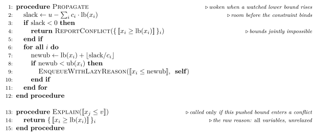
Algorithm 1. Linear propagator for \( \sum_i c_i x_i \le u \) in canonical form (all \( c_i > 0 \))
2.5 Lifting the reason
We kept the propagator deliberately simple: its Explain hands back the raw
row, the full set of bounds that were in force, without hunting for the smallest or
most general subset. CP-SAT makes up for that afterward. Conflict analysis
(Section 3.1) turns each reason into a permanent clause, and a
weaker reason, one that holds in more states, becomes a clause that rules out
more of them. So before learning, CP-SAT lifts the reason
(RelaxLinearReason): it spends the slack the deduction
left unused to loosen the bounds, recovering a more general clause than the
propagator literally reported.
Why is this sound? Because a push rarely uses all the room it had. Take the push of \( y \le 1 \), made when the slack was \( 8 \); reading off \( \lfloor 8/6 \rfloor = 1 \) gave \( y \le 1 \), but the leftover
\[ \ell \;=\; \big(\lfloor 8/6 \rfloor + 1\big)\cdot 6 \;-\; 8 \;-\; 1 \;=\; 2\cdot 6 - 8 - 1 \;=\; 3 \]
measures how much room was to spare. Forcing \( y \le 1 \) never needed the full bound \( z \le 8 \): even \( z \le 11 \) leaves \( y \ge 2 \) impossible once \( x \ge 0 \) is known, since \( 3\cdot 0 + 6\cdot 2 = 12 > 11 \). So CP-SAT lifts \( z \le 8 \) to \( z \le 11 \), weakening the bound by exactly \( \ell = 3 \), and conflict analysis resolves against the broader implication
\[ (x \ge 0 \;\wedge\; z \le 11) \;\Rightarrow\; y \le 1 \]
instead of the tighter \( z \le 8 \) form, learning a clause that can fire in more future states. The same trick broadens reported conflicts: there the slack is already negative, and its magnitude is the budget for loosening the bounds the violation did not strictly need.
All the propagator had to store to make this possible was a single integer, the leftover slack, carried alongside its claim check rather than a copied reason. That one number is what lets CP-SAT recover not merely a reason but a deliberately general one.
2.6 Expansion: which constraints keep a propagator
Section 2.4 said that every constraint type has a propagator. That is only half the story. A modeling language offers dozens of high-level constraints, and CP-SAT does not keep a bespoke propagator for each of them. During presolve, many constraints are expanded: rewritten into the small set of primitives that the engine reasons about natively, such as clauses, linear constraints, at-most-one constraints, and value literals. Only a curated subset is kept as dedicated global propagators.
Expanded away (cp_model_expand.cc):
Element,
Table (positive and negative),
Automaton/regular, and
Inverse. CP-SAT may also expand
AllDifferent heuristically when its domain
is small or close to a permutation; in that case, it becomes value literals plus
at-most-one constraints. Two more sit on a parameter-controlled line:
Reservoir is expanded by default (a
parameter can instead keep it native), while
LinMax constraints keep their propagator
by default, with a size threshold that opts only the small ones into
expansion.
The common thread is not that a stronger native propagator could never exist; it is that the decomposition is often cheap, exposes useful Boolean or value structure to the rest of the engine, or is competitive enough that a dedicated algorithm would not reliably pay for itself.
Kept as native propagators (cp_model_loader.cc): Boolean
constraints, loaded as clauses; linear constraints, crucially
with enforcement literals, that is, half-reified “indicator” constraints
in which a literal \( \ell \) enforces a linear constraint; integer product
(variable \( \times \) variable), division (the divisor may be a variable),
and modulo constraints (the modulus must be a fixed constant; a variable
modulus is decomposed into division and product during presolve);
AllDifferent on bounds when it is not a small permutation; Circuit and MultipleCircuit for routing; and the scheduling trio NoOverlap, Cumulative, and NoOverlap2d. These are the constraints whose specialized algorithms (edge-finding, energetic reasoning, subtour elimination, and Hall-interval pruning) can prune far more than any clause decomposition could. This is where the “CP” in CP-SAT does its real work.
This point is easy to oversimplify, so one nuance is worth stating plainly: the released code defaults to keeping native propagators, and expansion is gated by size heuristics and parameters rather than applied wholesale. The reason ties directly back to the cost argument of this part. A dedicated global propagator is expensive, so CP-SAT keeps it only where its extra pruning tends to pay for itself; everything else is handed to the cheap, always-on clause and linear machinery.
2.7 Search: guessing when propagation stalls
Whether a constraint reasons through a native propagator or an expanded decomposition, propagation eventually runs dry: it reaches a fixed point with nothing left to deduce. If every variable happens to be fixed, that fixed point is a solution. Usually it is not. With no conflict, the fixed point may still leave \( 3 \le x \le 7 \) open: if every constraint is satisfiable across that whole range, no propagator has any reason to tighten it. That is a consistent state, but not a solution. A solution must assign \( x \) one concrete value, and propagation alone, which only ever draws forced conclusions, cannot supply it. Closing the gap falls to search.
The solver’s only move at a stalled fixed point is to guess. The guess is a decision: it asserts a single literal, for instance trying \( [\![x \le 7]\!] \) true, with its negation \( [\![x \ge 8]\!] \) held in reserve as the other branch. As Section 2.1 noted, an integer bound is itself a reified literal, so guessing \( [\![x \le 7]\!] \) and flipping a native Boolean are the same step, both recorded at a new decision level.
A decision sets off a fresh cascade of propagation, and the guess is judged by what that cascade returns: it may pin more variables and let the solver descend with another guess; it may fix everything with no conflict, giving a solution; or it may reach a conflict, proving the guess wrong and forcing the solver to backtrack and learn (Section 3.1). Decisions stack on the trail, each tagged with its decision level, and backtracking pops them off and relaxes the bounds they imposed. Search is then just this loop: guess a literal, let the resulting cascade say whether it was right, wrong, or simply not yet decisive, and guess again until every variable is pinned. How the solver picks each literal, and what it does once the Booleans are all assigned but an integer still spans a range, is the search machinery assembled in Section 5.3.
3 Learning from failure
Every propagator in Section 2 can already report why it made each deduction: the reason behind each pushed bound. So far that capability has gone unused, ready on every push but never once invoked. This section is where it pays off. When propagation hits a dead end, those reasons let the solver dissect the failure, trace it back to the handful of decisions truly responsible, and distill that into a permanent rule, a single cheap clause, it never violates again. That is the faculty separating CP-SAT from classical CP, and the SAT half of the solver: turning a single failure into knowledge instead of undoing it and forgetting.
3.1 Conflict analysis and learning: the SAT half
This is where CP-SAT departs from textbook CP, and where lazy clause generation lives. When propagation derives a conflict, a plain CP solver would simply undo the last decision and try the other branch. CP-SAT instead asks why the failure happened, performing conflict analysis.
The mechanism that makes this possible is that every bound a propagator pushes comes with a reason: the set of facts that forced it. When the \( x + y \le z \) propagator deduced \( x \le 2 \), its reason was “\( z \le 4 \) and \( y \ge 2 \).” A reason is, in essence, an implication:
\[ (z \le 4 \;\wedge\; y \ge 2) \;\Rightarrow\; x \le 2 . \]
These implications chain. When a conflict surfaces, the solver walks backward through the reasons of the bounds involved, resolving them together until it isolates a compact subset of decisions that is jointly responsible. From that subset it builds a learned clause: a nogood that says, in effect, “never again let all of these conditions hold simultaneously.”
Three consequences follow, all inherited from CDCL SAT:
- The learned nogood is persistent until it is deemed unhelpful and garbage-collected. It prunes not just this branch, but every future branch where the same combination would recur, possibly in a completely different part of the search tree.
- Backjumping replaces chronological backtracking. Conflict analysis identifies the real culprit decision level, which may be far above the current one. The solver jumps straight back there in one step, undoing the intervening decisions and their propagations wholesale rather than retrying them level by level. This is far more powerful than the one-level-at-a-time backtracking of classical CP.
- The learned clause itself propagates. After backjumping, the new nogood immediately forces a bound, redirecting search productively instead of merely retrying.
The phrase “lazy clause generation” captures the efficiency trick underneath: the implications justifying each deduction are not eagerly written out as stored Boolean clauses. A propagator’s reason is assembled on the spot when conflict analysis asks for it, resolved into the learned clause, and otherwise left implicit. The overwhelming majority of deductions are made, used, and undone on backtracking without any clause ever materializing; the solver pays that cost only for the facts that turn out to matter for learning. Carrying reasons is what makes this correct: a learned clause is sound only because its literals are exactly the facts that forced the conflict.
Figure 2 shows this on a Sudoku: a single guess empties one cell’s domain, and walking the eliminations backward pins the blame on only two of the seven guesses, so the solver learns a nogood over those two and backjumps past the rest. The worked trace below makes the same steps precise on an integer model, where each struck candidate becomes a Boolean bound literal.
3.2 A worked conflict-analysis trace
To make Section 3.1 concrete, here is a step-by-step trace of one 1-UIP derivation on a small integer model, following the resolution CP-SAT performs (ComputeFirstUIPConflict).
The model. Take six non-negative integer variables \( x_1, \dots, x_6 \) and four linear constraints:
\[ C_0:\ x_6 \ge x_1 + x_2, \quad C_1:\ x_4 \ge x_3 + 1, \quad C_2:\ x_5 \ge x_4 + x_2, \quad C_3:\ x_4 + x_5 \le 9 . \]
The constraints are kept small so that each propagation step is a single line of integer arithmetic and the resolution can be followed by hand.
The search so far. Suppose the solver has already branched to \( [\![x_2 \ge 2]\!] \) (level 1) and \( [\![x_1 \ge 3]\!] \) (level 2). With both bounds in place, \( C_0 \) propagates \( [\![x_6 \ge 5]\!] \), since \( x_6 \ge x_1 + x_2 \ge 5 \). This bound is sound but turns out to be irrelevant: conflict analysis never walks through it. That is exactly the point of carrying reasons, rather than blaming every decision on the trail. The solver now branches a third time, to \( [\![x_3 \ge 4]\!] \) (level 3), and the current level cascades. Constraint \( C_1 \) propagates \( [\![x_4 \ge 5]\!] \) from \( x_4 \ge x_3 + 1 \ge 5 \), and this new bound feeds two constraints at once. Together with \( x_2 \ge 2 \) it drives \( C_2 \) to \( [\![x_5 \ge 7]\!] \), since \( x_5 \ge x_4 + x_2 \ge 7 \), while on its own it drives \( C_3 \) to \( [\![x_5 \le 4]\!] \), since \( x_5 \le 9 - x_4 \le 4 \). These two bounds cannot both hold, yet nothing in the four linear constraints says so directly; none of them mentions \( x_5 \ge 7 \) and \( x_5 \le 4 \) together. The incompatibility surfaces one layer down, in the Boolean model the bounds live in, whose bound literals are tied by consistency clauses that no user constraint wrote down. From \( [\![x_5 \le 4]\!] \) the monotone link \( x_5 \le 4 \Rightarrow x_5 \le 5 \) pushes \( [\![x_5 \le 5]\!] \), and that bound is what meets \( [\![x_5 \ge 7]\!] \). An upper bound is a lower bound’s negation, so \( [\![x_5 \le 5]\!] \) is \( \lnot[\![x_5 \ge 6]\!] \), while \( [\![x_5 \ge 7]\!] \) forces \( [\![x_5 \ge 6]\!] \). The bound literal \( [\![x_5 \ge 6]\!] \) is thereby driven both true and false: the empty domain on \( x_5 \), read at the Boolean level, is this clash. That is the conflict, and it is the underlying SAT model, not any propagator, that closes it.
Every derived bound has a reason, the facts that forced it, and conflict analysis resolves over those reasons whatever their source. Each reason is one of two things: a clause living directly in the SAT model, or a CP propagator’s explanation built lazily on demand. The SAT clauses include the ones Boolean constraints compile to, but also clauses no explicit constraint wrote down: the order-encoding consistency clauses that tie a variable’s bound literals together, and the nogoods learned from earlier conflicts. Here the failing clause is one of those implicit order-encoding clauses, the monotone link \( \{\lnot[\![x_5 \ge 7]\!],\ \lnot[\![x_5 \le 5]\!]\} \), whose second literal is the bound literal \( [\![x_5 \ge 6]\!] \) in disguise (\( [\![x_5 \le 5]\!] \) is its negation). Its literals are Boolean bound literals \( [\![\cdot]\!] \), the objects conflict analysis reasons over.
These reasons form an implication graph (Figure 3), and reading it backward from \( \bot \) is exactly the resolution that follows. The graph also shows why one decision is spared: \( x_2 \ge 2 \) forces two bounds, \( x_5 \ge 7 \), which reaches \( \bot \), and the off-path \( x_6 \ge 5 \), which does not. Walking back from \( \bot \) reaches \( x_2 \ge 2 \) through \( x_5 \ge 7 \) and never visits \( x_6 \ge 5 \), so the level-2 decision \( x_1 \ge 3 \), whose only role was to force that off-path bound, stays untouched.
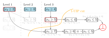
Figure 3. Implication graph for the trace: nodes are bound literals \( [\![\cdot]\!] \), blue for decisions and \( \bot \) for the conflict, with the rule that forced each propagated bound beneath it. The orange 1-UIP cut isolates the dominator \( x_4 \ge 5 \) and the lower-level decision \( x_2 \ge 2 \) (ringed), whose negation \( \{\lnot[\![x_4 \ge 5]\!],\ \lnot[\![x_2 \ge 2]\!]\} \) is the learned nogood; the faded branch is the off-path \( x_6 \ge 5 \) that analysis never visits.
The resolution. Before the walk, one convention is worth stating. Each
bound on the trail holds as a true fact, such as the \( x_4 \ge 5 \) the solver
set, whereas the clauses it appears in, both the failing clause and the reasons,
carry the corresponding negated bound literal. Resolving on \( x_4 \ge 5 \)
therefore means cancelling \( \lnot[\![x_4 \ge 5]\!] \) in the working
clause against \( [\![x_4 \ge 5]\!] \) in its reason. The
\( \text{Reason}(\ell) \) the loop calls is a dispatch, not a lookup in some shared
table: when a propagator enqueues a bound it stamps that trail entry with its own
identifier, so the trail records which propagator set each \( \ell \). Asking for
\( \text{Reason}(\ell) \) calls exactly that propagator back to explain its
deduction, building the justifying clause on demand and caching it
(Trail::Reason, which indexes propagators_
by the stored setter and invokes its Reason); decisions and unit facts
carry an empty reason and end the walk. This is the lazy clause generation of
Section 3.1 at work: the reason exists only once conflict analysis
asks the propagator that produced \( \ell \) for it. With this
convention in place, the algorithm keeps a working clause, initially the failing
clause, and repeatedly replaces the most recently assigned current-level bound by
its reason until exactly one current-level bound remains. It processes
bounds by decreasing trail index, which peels the conflict backward toward the
dominator. Formally, this is a short resolution loop:

Algorithm 2. First-UIP conflict analysis (ComputeFirstUIPConflict)
Walking that loop on our trail makes the mechanics concrete:
-
Start. The working clause is the failing clause, the order-encoding consistency clause \( \{\lnot[\![x_5 \ge 7]\!],\ \lnot[\![x_5 \le 5]\!]\} \): the monotone link \( [\![x_5 \ge 7]\!] \Rightarrow [\![x_5 \ge 6]\!] \), written with \( \lnot[\![x_5 \le 5]\!] \) in place of the bound literal \( [\![x_5 \ge 6]\!] \) it equals. Both bounds were assigned at the current level, level 3, so the loop continues.
-
Resolve on \( x_5 \ge 7 \) (highest trail index, position 5). Its reason is \( C_2 \) acting on \( x_4 \ge 5 \) and \( x_2 \ge 2 \), giving the clause \( \{\lnot[\![x_4 \ge 5]\!],\ \lnot[\![x_2 \ge 2]\!],\ [\![x_5 \ge 7]\!]\} \), which says that \( x_4 \ge 5 \) and \( x_2 \ge 2 \) together force \( x_5 \ge 7 \). Replacing \( \lnot[\![x_5 \ge 7]\!] \) by the rest of that reason (writing \( \odot \) for resolution) gives
\[ \begin{aligned} \{\lnot[\![x_5 \ge 7]\!],\ \lnot[\![x_5 \le 5]\!]\} &\odot \{\lnot[\![x_4 \ge 5]\!],\ \lnot[\![x_2 \ge 2]\!],\ [\![x_5 \ge 7]\!]\} \\ &= \{\lnot[\![x_5 \le 5]\!],\ \lnot[\![x_4 \ge 5]\!],\ \lnot[\![x_2 \ge 2]\!]\}. \end{aligned} \]
Two current-level bounds remain, \( x_5 \le 5 \) and \( x_4 \ge 5 \), so the loop continues.
-
Resolve on \( x_5 \le 5 \) (position 4). This is the order-encoding step: \( x_5 \le 5 \) was forced not by a constraint but by the monotone link \( x_5 \le 4 \Rightarrow x_5 \le 5 \), whose clause is \( \{\lnot[\![x_5 \le 4]\!],\ [\![x_5 \le 5]\!]\} \). Replacing \( \lnot[\![x_5 \le 5]\!] \) gives
\[ \begin{aligned} \{\lnot[\![x_5 \le 5]\!],\ \lnot[\![x_4 \ge 5]\!],\ \lnot[\![x_2 \ge 2]\!]\} &\odot \{\lnot[\![x_5 \le 4]\!],\ [\![x_5 \le 5]\!]\} \\ &= \{\lnot[\![x_5 \le 4]\!],\ \lnot[\![x_4 \ge 5]\!],\ \lnot[\![x_2 \ge 2]\!]\}. \end{aligned} \]
The bounds \( x_5 \le 4 \) and \( x_4 \ge 5 \) are both current-level, so the loop continues.
-
Resolve on \( x_5 \le 4 \) (position 3). Its reason is \( C_3 \) acting on \( x_4 \ge 5 \), giving the clause \( \{\lnot[\![x_4 \ge 5]\!],\ [\![x_5 \le 4]\!]\} \), which says that \( x_4 \ge 5 \) forces \( x_5 \le 4 \). Replacing \( \lnot[\![x_5 \le 4]\!] \) gives
\[ \{\lnot[\![x_5 \le 4]\!],\ \lnot[\![x_4 \ge 5]\!],\ \lnot[\![x_2 \ge 2]\!]\} \odot \{\lnot[\![x_4 \ge 5]\!],\ [\![x_5 \le 4]\!]\} = \{\lnot[\![x_4 \ge 5]\!],\ \lnot[\![x_2 \ge 2]\!]\}. \]
Only \( x_4 \ge 5 \) is now a current-level bound, since the other, \( x_2 \ge 2 \), belongs to level 1. Exactly one current-level bound remains, so the loop stops.
The UIP. The single remaining current-level bound is the first Unique Implication Point, \( x_4 \ge 5 \). It is the one node at level 3 through which every conflict path runs, since both \( x_5 \ge 7 \) and \( x_5 \le 5 \) were forced by it. Negating it and moving it to the front gives the learned clause
\[ \textbf{Learned nogood: } \{\lnot[\![x_4 \ge 5]\!],\ \lnot[\![x_2 \ge 2]\!]\}, \]
which reads “never have \( x_4 \ge 5 \) and \( x_2 \ge 2 \) at once,” or equivalently that whenever \( x_2 \ge 2 \) holds the bound \( x_4 \le 4 \) must follow. This is a fact stated purely in bounds, sound everywhere in the tree rather than only on this branch.
Backjump. The solver computes the assertion level: the highest decision level among the learned clause’s literals other than the UIP (ComputePropagationLevel). Here that is the level of \( x_2 \ge 2 \), namely level 1, so the solver retreats from level 3 straight to level 1. Everything above level 1 is undone in the process: the level-2 decision \( x_1 \ge 3 \) and its propagation \( x_6 \ge 5 \) are popped along with the level-3 cascade. Nothing in between is selectively kept; the undo is a plain truncation of both trails to the end of level 1, leaving only level 1 and below. The force of the non-chronological backjump is not that \( x_1 \ge 3 \) survives but that the solver does not stop at level 2 to retry it: that decision had no part in the failure, so search resumes at level 1 instead. One-level-at-a-time CP backtracking cannot make that jump.
Assertion. Back at level 1, \( x_2 \ge 2 \) is still true. So in the learned clause \( \{\lnot[\![x_4 \ge 5]\!],\ \lnot[\![x_2 \ge 2]\!]\} \) the literal \( \lnot[\![x_2 \ge 2]\!] \) is false and \( \lnot[\![x_4 \ge 5]\!] \) is the only unassigned literal. The clause is now unit and immediately propagates it, forcing \( x_4 \le 4 \) (AddLearnedClauseAndEnqueueUnitPropagation). Search resumes already knowing a fact that cost one conflict to learn, and that fact will fire automatically in every future branch where \( x_2 \ge 2 \) holds.
Two finishing touches CP-SAT applies in practice:
- Minimization. Before storing the clause, CP-SAT applies self-subsuming resolution (MinimizeConflict): any literal whose own reason is already implied by the other clause literals can be dropped, yielding a shorter, stronger nogood.
- LBD scoring. The clause’s LBD is recorded (ComputeLbd). Here the learned clause touches two distinct decision levels, so its LBD is 2. A low LBD marks it as a high-quality clause: it is more likely to be protected from clause-database cleanup, and it later feeds the restart heuristic (Section 6.3).
That one trace exercises every part of the engine: propagators deduce with reasons, the conflict resolves those reasons to a unique dominator, the dominator becomes a permanent learned clause, and a non-chronological backjump turns the lesson into immediate forward progress.
 In the solve log
Each conflict resolution increments the |
4 Lazy integer encoding
The conflict analysis of Section 3.1 resolved over Boolean bound literals such as \( [\![x_5 \ge 6]\!] \) and learned clauses written in them, taking for granted that those Booleans exist. This section describes where they come from: the part of CP-SAT that reconciles an integer variable with a huge domain with a CDCL engine that ultimately reasons in Boolean literals.
The lazy-reason machinery of the preceding sections only works because the Boolean layer it feeds is itself built lazily: an integer variable’s encoding into Booleans is created on demand, the same way its reasons are. That is why it follows learning directly rather than waiting among the later accelerators.
The encoding below puts one Boolean on each bound \( [\![x \ge v]\!] \), which looks like a unary encoding: a variable over a million values would seem to need a million Booleans, the very blow-up a binary encoding exists to avoid. The resolution is the word lazy. CP-SAT never lays down that unary chain in full; it mints a bound literal only at the moment some mechanism actually refers to it, so a wide integer typically contributes a handful of Booleans rather than its whole range. The encoding is unary in form but sparse in practice, and the rest of this section is about how that sparsity is achieved and what it costs elsewhere.
It also helps to be precise about what kind of mechanism this is. Lazy clause generation (Section 3.1) is a correctness mechanism: reasons are what make learned clauses sound deductions. Lazy encoding, by contrast, is an efficiency mechanism: CP-SAT would stay correct if it encoded every bound up front. Whether that would even hurt depends on the domains involved. Many models are dominated by Boolean variables, and a variable with a small domain costs only a few bound literals; there, eager encoding would do no real harm. The cost concentrates on the variables whose domains are genuinely wide. The objective is the usual one (a weighted sum can range over millions), and CP-SAT mints further wide-domain integers of its own when it breaks a long linear constraint into a tree of partial sums. Encode every bound of those up front and the model turns slow and memory-hungry.
4.1 Minting Booleans on demand
Why eager encoding is hopeless. The naive bridge would give every bound its own Boolean up front. A variable \( x \in [0, 10^6] \) would spawn a million literals
\[ [\![x \ge 1]\!],\quad [\![x \ge 2]\!],\quad \ldots \]
before search even starts. This is a non-starter in both memory and propagation cost, and the overwhelming majority of those literals would never be touched. CP-SAT therefore does not pre-encode all bounds. The integer trail reasons about bounds directly, as native integer facts (Section 2.1), and Booleans are created only where the integer and Boolean worlds actually need to meet.
The order encoding. When that bridge is built, it uses the order encoding, also called the “list encoding.” CP-SAT follows Feydy and Stuckey’s “Lazy Clause Generation Reengineered” (CP 2009) [10].
For a variable \( x \), the bound literals have the form \( [\![x \ge v]\!] \), and they are linked by the obvious monotone implications:
\[ [\![x \ge 6]\!] \;\Rightarrow\; [\![x \ge 5]\!] \;\Rightarrow\; [\![x \ge 4]\!] \;\Rightarrow\; \cdots . \]
A single such Boolean also represents the corresponding upper-bound fact, because
\[ [\![x \le v]\!] \equiv \lnot[\![x \ge v{+}1]\!] . \]
In the implementation, the upper-bound side is handled by sharing the encoding
with NegationOf\( (x) \), so \( x \) and its negation do not duplicate Booleans.
On-demand creation. The workhorse is GetOrCreateAssociatedLiteral\( (x \ge v) \). It returns the Boolean \( [\![x \ge v]\!] \). If that literal does not yet exist, it mints a fresh Boolean variable and wires in the implications to the already encoded neighboring bounds, the next bound below and the next bound above. This preserves the monotone chain.
This is the moment alluded to in the conflict trace of Section 3.2.
When 1-UIP resolution needs \( [\![x \ge v]\!] \) as a clause literal, this call
materializes it. The implication links keep it consistent
with its neighbors, and from then on the SAT engine treats it like any other
Boolean literal. In the basic search loop, two moments dominate bound-literal
creation: branching on an integer bound mints the Boolean for that
bound (GetDecisionLiteral), and
integer conflict resolution mints the Boolean it needs for the 1-UIP
(Section 3.2). Other mechanisms call the same
GetOrCreateAssociatedLiteral on demand as well, including core-guided
optimization when forming assumption literals, the feasibility pump, and some
global propagators. Ordinary bound propagation, however, stays in integer-bound
space and creates no Booleans. That is what keeps the Boolean skeleton small.
Equality literals. Some constraints, for example a table constraint, AllDifferent, or anything that reasons about exact values, want \( [\![x = v]\!] \), not just bounds. GetOrCreateLiteralAssociatedToEquality\( (x, v) \) provides it, based on the identity
\[ [\![x = v]\!] \;\Longleftrightarrow\; [\![x \ge v]\!] \;\wedge\; [\![x \le v]\!] . \]
A constraint may even ask for the whole domain at once via FullyEncodeVariable. This is the deliberate eager path, used precisely when a propagator is going to need every value anyway, so laziness would only add overhead. Full encoding is the exception requested by a constraint; lazy bound encoding is the default for everything else.
There is an important asymmetry between the two encodings. The bound literals
\( [\![x \ge v]\!] \) of the order encoding are predominantly dynamic: they
are minted during branching and conflict resolution as just described. Value
literals \( [\![x = v]\!] \) are predominantly static: the
equalities a model needs are detected and created up front during
presolve/loading (ExtractEncoding), rather
than on demand. That said,
GetOrCreateLiteralAssociatedToEquality can still mint one lazily if a
constraint later asks for a value literal that loading did not foresee. The
developers’ rule of thumb behind this split is blunt: if a model genuinely needs
per-value Booleans for a variable, that variable probably should not have been a
wide integer in the first place.
Domains with holes. Real domains are not always intervals. If \( x \in [1,2] \cup [5,6] \), then “\( x \le 3 \)” and “\( x \le 4 \)” mean the same thing as “\( x \le 2 \),” and “\( x \ge 3 \)” means “\( x \ge 5 \).” The encoder’s Canonicalize step folds each requested bound onto the canonical bound for that domain before looking it up. Equivalent bounds therefore share one Boolean instead of spawning redundant ones.
The payoff. The Boolean skeleton that the CDCL engine actually sees
stays small: it contains only the bounds and equalities that branching,
conflict learning, or a constraint-specific encoding genuinely reached. A
variable over a million values typically contributes a handful of literals, not
a million, and the encoder tracks exactly how many Booleans it had to create
(num_created_variables_). Both layers are lazy: the reasons
(Section 3.1) and the Boolean variables they are written in.
Strong integer propagation does
the bulk of the reasoning natively over bounds, and the Boolean encoding
materializes only at the thin interface where the learning machinery needs to
grip.
|
In the solve log
The size of the lazily minted Boolean skeleton is reported per worker as the
|
4.2 A fixed skeleton need not be a solution
The sparse skeleton has a consequence the foundational search of Section 2.7 sidestepped. Because the skeleton holds only a handful of bounds, all of them can be assigned while an integer still spans a range: \( [\![x \ge 3]\!] \) true and \( [\![x \ge 8]\!] \) false leave \( x \in [3,7] \) with every existing literal decided. The gap is then a missing literal, not an unassigned one. Even a complete Boolean assignment can leave \( x \) genuinely ranged, because no bound between \( 3 \) and \( 7 \) was ever minted. Under a full encoding this could not arise, since deciding every bound pins the value; the sparse skeleton is exactly what pulls the two tests apart.
Closing this gap is the job of integer completion, the second half of the search machinery in Section 5.3: once the Boolean skeleton is settled but some integer is still ranged, the solver mints a fresh bound for that integer and branches on it, repeating until every variable is pinned to a single value.
5 Putting it together
This section assembles the moving parts into a single control loop: bounds and their literals (Section 2), propagators that tighten them, branching that commits values, and conflict analysis that learns from failure (Section 3). It then opens the loop’s two busiest lines: what “propagate to a fixed point” actually runs, and in what order the SAT and CP engines take turns (Section 5.2); and how the next decision is chosen once propagation stalls, where a deliberate design choice has CP-SAT drive the search itself and lets a configurable decision strategy, by default led by SAT branching, choose where to descend (Section 5.3).
5.1 The search loop, assembled
Putting the pieces together, the engine is a single feasibility loop (SolveIntegerProblem, entered through the level-\( 0 \) reset-and-assert wrapper ResetAndSolveIntegerProblem) wrapped by a thin optimizer that calls it repeatedly. The loop, Solve (Algorithm 3), is the heart: every concept introduced so far appears in it exactly once, and each line points to a section that expands it. It takes a set of assumptions (literals forced true for the duration of one call) and returns either a feasible solution or a proof that none exists under them. The wrapper, MinimizeByBisection (Algorithm 4), turns that feasibility engine into an optimizer: it calls Solve under a trial bound on the objective and narrows that bound by bisection until the optimum is pinned.
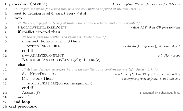
Algorithm 3. The CP-SAT feasibility core, Solve
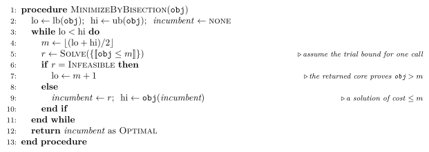
Algorithm 4. Optimization by bisection: MinimizeByBisection drives Solve
The two procedures factor the engine cleanly. Solve’s contract is feasibility: it returns a feasible assignment or a proof none exists, and it never manages the objective bound — that bookkeeping is entirely the wrapper’s. The loop itself carries no optimization logic; the only cost-awareness inside it lives in the decision strategies, which can be set up, explicitly or implicitly, to branch toward cheaper solutions (Section 5.3). MinimizeByBisection (RestrictObjectiveDomainWithBinarySearch) keeps a lower and an upper bound on the optimal cost and, each round, asks Solve whether a solution of cost at most the midpoint \( m \) exists — forcing the order-encoding literal \( [\![\, \texttt{obj} \le m \,]\!] \) (minted on demand by GetOrCreateAssociatedLiteral) as an assumption, a fact held only for that one call. This works because the objective is just one more bounded integer variable (Section 5.5) and a bound is a literal (Section 2). The two answers move opposite ends of the gap: a solution pulls the upper bound down to its cost, while an Infeasible hands back a core — the subset of the assumptions that cannot hold together — proving \( \texttt{obj} > m \) and lifting the lower bound. When the two bounds meet, the incumbent is optimal, and that final infeasibility proof is the proof of optimality. This is the first place Solve’s assumption input and core output earn their keep; Section 5.5 puts the same \( A \) parameter to work in the other strategies that drive this loop.
This single loop hides a deeper design decision: how the CDCL clause-learning machinery is coupled to finite-domain propagation. There are broadly two ways to wire the two together. One option is to keep a complete CDCL SAT solver in charge and let it own the whole search stack: the trail, the decisions, unit propagation, conflict analysis, and backjumping. The finite-domain side then talks to it only through the clause interface, injecting fresh clauses (and the Boolean variables they need) whenever it notices the solver has missed something a constraint implies. The SAT engine runs the show; the constraint reasoning feeds it from outside.
CP-SAT takes the other option: it drives the search itself. It runs its own propagation, conflict analysis, and search as one integrated core, and the CDCL clause-learning machinery is a mechanism inside that core rather than an external engine being fed from the side. This choice runs through every line of the loop. Boolean literals and integer bounds share one decision-level timeline across two coupled trails (Section 2.2), so the PropagateToFixedPoint step runs the CP propagators directly and a finite-domain propagator pushes an integer-bound fact onto the integer trail itself (Section 5.2); conflict analysis then resolves over those integer literals natively, and the Boolean clauses and variables are minted lazily, only at the thin interface where the two worlds meet. This is what lets the costly apparatus of Section 3 pay off: a decision and the reason later learned from it are written in the very same literals, so every failure feeds straight back into the search that produced it, with no re-encoding round trip.
The interesting work inside Solve’s conflict case is split between learning and backjumping. Branching is not a single rule but a walk down an ordered decision strategy \( \mathcal{S} \), a list of heuristics: NextDecision tries each in turn and returns the first literal one produces, which the loop then asserts. By default \( \mathcal{S} \) holds two such heuristics (Section 5.3): the SAT decision heuristic (VSIDS), which keeps branching on existing bound literals until every one has a value, and integer completion, a generic fallback that takes the first variable still spanning a range and fixes it toward its minimum. Running only after VSIDS has settled every Boolean, completion in practice sees just the integers the skeleton has left loose, minting one bound at a time until each domain collapses to a single value. The loop reports a solution only when every heuristic in \( \mathcal{S} \) comes up empty, which is why the leaf test is stricter than “all Booleans assigned”: it holds only once every domain has also shrunk to a singleton.
Which heuristics \( \mathcal{S} \) contains, and in what order, is part of the configuration rather than a fixed feature of the loop. Section 5.3 takes the strategy apart: what each of the two default heuristics does, and how the parallel portfolio reorders and extends them across workers.
|
In the solve log
Each pass through the Assert line is counted as a |
Solve and its optimizer, together with strong propagators, are the search core. Bisection is one clean way to drive the feasibility loop; Section 5.5 surveys the others, including the even simpler linear scan and the core-guided strategies the portfolio runs.
5.2 Inside “propagate to a fixed point”
The loop of Section 5.1 hides its most important line: “propagate to a fixed point.” What actually happens there, and where does the SAT engine sit relative to the CP propagators?
 Not generate-and-check CP-SAT does not let the SAT solver guess a complete Boolean assignment and then hand it to the CP propagators for checking, as in generate-and-check lazy SMT or CEGAR. Propagation is online: it runs after every decision, before the next one, and the propagators always operate on the current partial state, namely the bounds as they stand, never on a finished assignment. |
A layered, cheapest-first cascade. Propagators are kept in a fixed order, with the cheapest and most prolific first, and the engine runs them as a chain:
- the binary-implication graph: implications from two-literal clauses, the cheapest form of unit propagation;
- the clause manager: unit propagation on general clauses via the two-watched-literals scheme;
- enforcement and pseudo-Boolean constraints;
- the GenericLiteralWatcher, which fans out to all integer and CP propagators: linear, AllDifferent, NoOverlap, Cumulative, and so on.
The first two layers are classical SAT unit propagation. This is the “first-row propagator” picture: cheap, always-run Boolean reasoning fires before any expensive global constraint is even consulted.
Restart-on-progress is the key scheduling rule. The instant any propagator deduces something new, by enqueuing a literal or tightening a bound, the chain breaks and starts again from the top. Thus, when an expensive global constraint such as Cumulative tightens a bound, control immediately returns to binary-implication and clause unit propagation. Those cheap layers then run to their own fixed point again before any expensive propagator is reconsidered. Cheap reasoning is always exhausted before the engine spends time on expensive reasoning.
The same discipline repeats one level down inside GenericLiteralWatcher. CP propagators are themselves bucketed by priority: priority 0 for cheap propagators such as linear and scheduling helpers, and higher priorities for more expensive propagators such as AllDifferent or Cumulative. The watcher drains priority 0 before priority 1, but resets to priority 0 as soon as a cheap propagator tightens a bound. If a propagator pushes a Boolean literal, control returns to the SAT layer immediately, so unit propagation re-runs before anything costlier.
Change-driven waking. None of this rescans every constraint in every round. At registration, a propagator declares exactly which literals and variable bounds it cares about (WatchLiteral, WatchLowerBound, WatchUpperBound). It is then woken only when one of those facts changes, and it receives the changed watch indices through IncrementalPropagate rather than recomputing from scratch. The fixed-point loop is therefore sparse: only the constraints touched by the last deduction are re-run, and they are usually told precisely what moved.
Putting this together, a single decision triggers a cascade that first exhausts the cheapest propagation, escalates to expensive global constraints only when the cheap layers stall, returns to cheap propagation the moment anything new is deduced, and wakes only constraints whose watched facts changed. Only when the entire cascade stalls does control return to branching; if some propagator instead empties a domain, control goes to the conflict analysis of Section 3.1.
|
In the solve log
The two trails are tallied by two separate columns of the Search stats
table. |
5.3 Inside “search”: choosing the next decision
The companion to “propagate to a fixed point” is the other line the loop hides: how the next decision is actually chosen. The integrated design of Section 5.1 — one decision-level timeline across its two trails, with clause learning a mechanism inside the core — settles how decisions are represented and learned from, but not which heuristic picks the next one. That is the configurable decision strategy \( \mathcal{S} \) of Section 5.1: the default leads with SAT branching and falls back to finite-domain branching, but other workers reorder these or lead with an LP or a fixed integer order instead. The two heuristics below are the entries of that default \( \mathcal{S} \), and the building blocks the other strategies recombine.
The SAT decision heuristic. This entry branches on a bound literal that
already exists. CP-SAT’s SAT core chooses it by VSIDS
(sat_decision.h:58): it keeps a decaying activity score per variable,
bumps the variables that appear in each conflict, and branches on whichever has
been most involved in recent failures, with a saved polarity (phase
saving) picking true or false. Because an integer bound is a reified literal
(Section 2.1), this one heuristic ranges over Boolean and integer
variables alike: the literals it scores are exactly the bound literals conflict
analysis has been resolving over. This is the sense in which this entry branches
from the SAT side.
Integer completion. VSIDS can branch only on literals that already
exist, and the sparse skeleton (Section 4.2) lets those run out
while an integer is still ranged: every existing bound for \( x \) is assigned,
yet \( x \in [3,7] \) because no bound between \( 3 \) and \( 7 \) was ever minted. When
the SAT heuristic reports nothing left to decide, every Boolean is assigned
(SatSolverHeuristic), and only then does an
integer-completion heuristic step in: it picks a still-ranged variable,
mints a fresh bound for it, and branches on that. The default composition puts
completion last for exactly this reason (integer_search.cc:1224):
exhaust the existing Booleans first, and fall back to minting a new one only when
the skeleton is settled but some integer is still loose.
Which bound to mint is a value-selection choice. The default branches the variable toward its current minimum, asserting \( [\![x \le \text{lb}(x)]\!] \) (AtMinValue): the first guess tries the smallest surviving value, and the other branch pushes the lower bound up. Other configurations bisect instead, minting a middle bound \( [\![x \ge \text{lb} + \lceil(\text{ub}-\text{lb})/2\rceil]\!] \) (GreaterOrEqualToMiddleValue) to halve the range per decision, or split around the current LP value. Each is just a rule for which not-yet-minted bound becomes the next decision.
This is why search terminates on \( \text{lb} = \text{ub} \) rather than when the Booleans are exhausted: completion keeps minting bounds for an unfixed variable instead of declaring victory once the SAT skeleton is satisfied. The propagation fixed point of Section 5.2 becomes a solution only when every integer has been pinned to a single value, one missing literal at a time.
How workers vary the strategy. These two heuristics are only the default
\( \mathcal{S} \). Nothing in the loop of Section 5.1 fixes which
strategy it runs, and the parallel portfolio (Section 6.4)
exploits this, running workers whose \( \mathcal{S} \) differs in both contents and
order, selected through the search_branching parameter:
auto(AUTOMATIC_SEARCH, the default): \( \langle\text{VSIDS},\ \text{integer completion}\rangle \);fixed(FIXED_SEARCH): \( \langle\text{fixed integer order},\ \text{VSIDS}\rangle \), the integer-style decisions first, with VSIDS only settling any leftover Booleans;reduced_costs(LP_SEARCH): \( \langle\text{LP reduced-cost},\ \text{VSIDS},\ \text{integer completion}\rangle \);pseudo_costs(PSEUDO_COST_SEARCH): \( \langle\text{pseudo-cost},\ \text{VSIDS},\ \text{integer completion}\rangle \);portfolioandquick_restart(PORTFOLIO_SEARCH, PORTFOLIO_WITH_QUICK_RESTART_SEARCH): a randomized rotation over such lists, reshuffled on restart.
Only the contents and order of \( \mathcal{S} \) change between workers; the loop around it does not.
 Tuning the search
You can also supply your own search strategy \( \mathcal{S} \) instead of leaving it to the
portfolio. The search_branching parameter (default |
5.4 A small worked example
The following tiny model illustrates the control loop without introducing an objective yet:
\[ \begin{aligned} &a, b, c \in \{0, 1\} \quad\text{(Booleans)}, \qquad x \in [0, 5] \\ &\text{C1:}\ a + b + c \ge 2 \quad\text{(at least two of } a,b,c \text{ are true)}\\ &\text{C2:}\ x \ge 3a \\ &\text{C3:}\ x \le 2 \end{aligned} \]
Root propagation. C3 tightens \( x \) to \( x \le 2 \). C2 says \( x \ge 3a \); in combination with \( x \le 2 \), it forces \( a = 0 \), because \( a = 1 \) would require \( x \ge 3 \). Now C1 becomes \( b + c \ge 2 \), forcing \( b = 1 \) and \( c = 1 \). All of this is pure deduction, with no decisions at all.
Completion search. At this point the state is consistent, but not yet a solution. The Boolean variables are fixed, whereas \( x \) still ranges over \( [0,2] \): once \( a=0 \), no remaining constraint distinguishes \( x=0 \), \( x=1 \), and \( x=2 \). Recall Section 5.3: search terminates only when every variable has a singleton domain. The completion brancher therefore still takes a decision on \( x \). Under the minimum-first completion heuristic, it tries \( x \le 0 \); together with the existing lower bound \( x \ge 0 \), this fixes \( x=0 \). Only then is the total assignment \( (a,b,c,x) = (0,1,1,0) \) reported.
The example is intentionally conflict-free. Its purpose is to show the ordinary case in which propagation and branching cooperate: propagation performs the forced deductions, and search supplies the remaining choices needed to turn a consistent state into a complete assignment. If a later decision in another branch did lead to a conflict, the same reasons attached to these propagations would feed the conflict analysis described in Section 3.1.
5.5 Optimization: solving feasibility, repeatedly
Optimization treats the objective as one more bounded integer variable. This is
literal, not a metaphor: the model holds a dedicated integer variable,
objective_var, constrained to equal the
objective expression, and to
minimize is to drive down its upper bound. Because it is an ordinary integer
variable, it sits on the integer trail, propagators watch and tighten it, and
parallel workers share improved bounds on it like any other bound
(Section 6.4). This is what lets MinimizeByBisection
(Algorithm 4) optimize with no optimization-specific search: it
only ever moves a bound on objective_var and re-runs the same feasibility
loop. Bisection is one way to move that bound; it is not the only one.
Linear scan (optimization.cc:212) is even simpler, and it is the
one strategy that needs no assumptions at all. Find a solution of cost \( C \), then forbid that cost and
everything worse and search again. Because the objective only ever has to improve,
the cutoff is monotone: it never has to be taken back. So rather than
assuming it for a single call, MinimizeByLinearScan permanently
tightens objective_var’s upper bound to \( C - 1 \) at the root
(Algorithm 5); the bound becomes part of the model, propagates like
any other, and every later solution is strictly cheaper. When the tightened model
is infeasible, the last \( C \) was optimal — again the infeasibility proof is
the proof of optimality. This is the contrast with bisection that matters: bisection
probes a bound it may have to retract, so it assumes it; linear scan tightens
a bound it will never relax, so it asserts it for good. Either way, CP-SAT
reports both an incumbent (the best feasible cost so far) and a
bound (the best cost ruled out below); when the two meet the gap is zero
and optimality is proved, and good incumbents, propagating like any other bound,
accelerate that proof.
|
The step size comes from the search, not the cutoff The cutoff posted after each solution only demands that the next one be strictly better: it tightens \( [\![\, \texttt{obj} \le \texttt{obj}(\textit{incumbent}) - 1 \,]\!] \), a single unit. How far each step actually moves is set by the search, not by that cutoff. Objective-directed decision strategies, such as branching toward the LP relaxation’s values (Section 5.3), steer each Solve call toward a good assignment rather than merely a feasible one just under the cutoff, so the solution returned is usually much cheaper than one unit better. Linear scan therefore tends to descend in large, uneven jumps rather than crawling unit by unit. The same effect helps bisection: it banks the returned incumbent’s true cost (Algorithm 4, \( \text{hi} \gets \texttt{obj}(\textit{incumbent}) \)), which often sits well below the probed midpoint. |
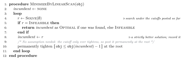
Algorithm 5. Linear scan: MinimizeByLinearScan tightens a monotone bound
Core-guided workers
(CoreBasedOptimizer) push the same machinery
further. Instead of bounding
obj as a whole, they assume the individual objective terms at their best
values and call Solve; each returned core
(FindCores) is a set of terms that cannot
all stay at their best, which they use to reformulate the objective and lift the
lower bound (sometimes minimizing the core first). Bound-focused workers
(objective_lb_search, objective_shaving) specialize in the dual
side. They differ in how they move the incumbent and the bound, but every
one of them is an outer loop over the single Solve of
Algorithm 3: they share its propagation, learning, and search, and
vary only what they assert or assume on the objective between calls.
|
In the solve log
The optimizer’s bound-tightening is what generates the streaming progress lines: each
improving incumbent prints as |
6 Going faster
Everything up to here is enough to explain the correctness of the core: in an unlimited exact run, the solver of Sections 2–5 finds optima and proves them. This section is about being fast. Each technique that follows is an accelerator layered onto that same core: the LP relaxation, cutting planes, restarts, and the parallel portfolio. In the idealized complete-search sense, these do not change the feasible set or the optimum; in practical time-limited runs, they can of course change whether CP-SAT proves optimality, returns only an incumbent, or times out without a useful solution.
|
Background The accelerators in this section all run during search. CP-SAT also spends a considerable effort before search begins, on presolve: a preprocessing pass that simplifies and canonicalizes the model, removes redundant variables and constraints, tightens bounds, and expands high-level constraints into the primitives the search core understands. None of it is exotic, but it is fundamental to performance, and a model often shrinks dramatically before a single decision is made. We leave presolve out of scope here; the general ideas, drawn from the SAT and MIP traditions CP-SAT inherits, are covered in lectures on SAT and MaxSAT preprocessing [11, 12] and in Achterberg et al.’s survey of MIP presolve reductions [13]. |
6.1 The LP relaxation: dual simplex as a propagator
Pure constraint propagation reasons one constraint at a time. It is weak exactly where linear programming is strong: at providing a global numeric view of all linear constraints at once, a sharp lower bound on the objective, and reduced-cost arguments. CP-SAT therefore carries a continuous LP relaxation of part of the model alongside the search and uses it as one more propagator. This is the bridge to the MIP world, and it is where the dual simplex enters. The developers’ own account of these MIP aspects is a useful companion here [14].
It is just a propagator. LinearProgrammingConstraint implements the same PropagatorInterface as the CP propagators and registers with the GenericLiteralWatcher. It registers at a high-cost priority, so the cheapest-first rule of Section 5.2 runs it only after unit propagation and the light CP propagators have reached their fixed point. It watches integer-variable bounds (Booleans included, through their \( \{0,1\} \) integer views) and the objective bound, wakes incrementally when those bounds change, and, like any propagator, feeds its deductions back as integer-bound tightenings on the trail. Nothing in the search core changes; the LP is simply an unusually powerful propagator.
What it relaxes. CP-SAT loads the model’s linear constraints into a
continuous LP over the same variables, drops integrality, and uses each
variable’s current \( [\text{lb}, \text{ub}] \) as its column bounds. How much of the
model enters the LP is governed by linearization_level: level 0 means no
LP at all; level 1 adds the linear constraints together with the integer and
at-most-one encodings; and level 2 linearizes more aggressively still, pulling in
additional Boolean and reified structure and enabling the cut generators of
Section 6.2 where they apply. The proto documents only this coarse
0/1/2 progression; the precise set of relaxations admitted at each level is an
implementation detail and shifts between releases. This single knob is what
distinguishes the no_lp (0), default_lp (1), and max_lp
(2) workers of the portfolio (Section 6.4).
Why the dual simplex. This is the crux. Branching and propagation change
only variable bounds, the column bounds of the LP; they do not change the
constraint matrix or the objective. After such a bound change, the previous
optimal basis often remains dual-feasible, because dual feasibility depends on
the matrix and objective, while primal feasibility may be broken by the new
bounds. This is the textbook situation for the dual simplex: starting
from the saved basis, it repairs primal feasibility, typically in a small number
of pivots, instead of re-solving from scratch. CP-SAT sets
use_dual_simplex(true) and saves and reloads Glop’s basis state across
calls (GetState / LoadStateForNextSolve). This warm start is what
makes it affordable for an LP to sit inside a CDCL search.
What it gives back. The LP returns three kinds of deduction, each handed to the engine as ordinary integer-bound facts, or as a conflict, on the trail:
- A conflict, when the LP is infeasible. If the relaxation has no feasible point, CP-SAT can use a dual ray, a Farkas certificate, to form a linear combination proving that the current bounds are jointly impossible. That proof is reported as a learned conflict like any other (PropagateExactDualRay).
- A dual bound on the objective. When the LP is optimal, its value is a valid lower bound, for minimization, on the relaxation and therefore on the integer problem. The propagator pushes \( \text{objective\_var} \ge \lceil \text{lp\_objective} \rceil \), directly strengthening the bound that drives the optimality proof of Section 5.5.
- Reduced-cost strengthening. Given the incumbent cutoff, i.e., the objective’s current upper bound, each variable’s LP reduced cost says how much moving it away from its LP value would worsen the objective. If that movement would breach the cutoff, the variable’s domain can be tightened. This is classic MIP reduced-cost fixing, returned as ordinary integer-bound deductions.
Soundness despite floating point. The simplex runs in floating point,
which a solver that must be exact and must produce learnable
reasons cannot trust directly. CP-SAT therefore does not blindly believe the
LP’s numerical values; it treats them as proposals. For LP-derived deductions, it
scales the relevant dual multipliers to integers, using a power-of-two scaling
and then dividing by the gcd, and forms an exact integer linear combination of
the constraints. The result is a Farkas-style certificate that yields a provably
valid bound together with an exact reason expressed in integer bound literals.
That certified reason is what is enqueued and, if a conflict follows, learned.
With use_exact_lp_reason on by default, the deductions are exact
even though the LP that suggested them was approximate. This is what keeps the
LP compatible with lazy clause generation: the LP proposes, exact integer
arithmetic certifies, and the certified reason is there for CDCL when the
deduction enters conflict analysis.
Cost and throttling. A simplex re-solve is far heavier than an ordinary
propagator, so CP-SAT throttles the LP beyond merely assigning it a low priority.
At the root, it may be skipped unless enough deterministic time has elapsed since
the previous solve; pivot counts are capped per call; and the LP can be disabled
outright during heavy phases such as probing. The portfolio hedges this
trade-off directly: some workers pay nothing for the LP (no_lp), whereas
others pay for a maximal relaxation (max_lp), so the ensemble covers both
sides of the bet on whether the linear structure is worth the cost.
In short, the LP injects the kind of reasoning that constraint propagation cannot provide on its own: a global, dual-certified numeric bound. It does so without disturbing the engine. It is a propagator, woken by bound changes, that returns exactly justified bound tightenings, made affordable by dual-simplex warm starts.
|
In the solve log
Every LP-bearing worker adds a row to the Lp stats table:
|
6.2 Cutting planes: tightening the relaxation
The LP of Section 6.1 is only as strong as the constraints in it, and the bare relaxation of an integer model is often loose.
Presolve already buys some tightening for free: coefficient strengthening rewrites a coefficient that the right-hand side leaves partly slack into a tighter one, without changing the set of integer solutions. The source’s own example is \( 3x + 5y \le 6 \) with \( x, y \in \{0,1\} \): the coefficient \( 5 \) can be raised to \( 6 \), since \( y = 1 \) already forces \( x = 0 \) either way, so no integer point is lost while the linear relaxation becomes sharper at no extra row. True to the engine’s preference for Boolean structure, CP-SAT can even re-express such a constraint through an enforcement literal when one is implied.
Cutting planes sharpen the relaxation further. They are extra linear
inequalities that every integer solution satisfies but that the current
fractional LP optimum violates. Adding them cuts off the fractional point without
removing any feasible integer point, so the next re-solve can return a tighter
dual bound. This is the MIP half of CP-SAT: cuts are generated into the same
shared LP and gated by the linearization_level of Section 6.1.
Generic MIP cuts. From the LP basis, CP-SAT separates standard cut families: Chvátal–Gomory cuts, with multipliers read from \( B^{-1} \); MIR cuts, mixed-integer rounding cuts obtained by combining a few tight rows; zero-half cuts, based on a mod-2 heuristic; and knapsack/cover cuts with lifting. It also derives implied-bound and clique cuts from the Boolean structure.
One recipe behind many of them. Despite the different names, many
generic cuts follow the same four-step pattern (cuts.cc).
(1) Aggregate. Take a linear combination of LP rows (the same algebraic operation behind the LP’s reasons in Section 6.1) to obtain a single constraint that is tight, or nearly tight, at the current fractional point. The multipliers distinguish the families: Chvátal–Gomory reads them from a row of \( B^{-1} \), MIR combines only a handful of rows, and zero-half uses small coefficients such as \( \pm 1 \).
(2) Rewrite. Put the aggregate into a canonical form over non-negative variables, complementing some variables (\( x \mapsto \text{range}-x^c \)) and substituting implied bounds so that the rounding step is valid.
(3) Round. Apply a super-additive function \( f:\mathbb{Z}\to\mathbb{Z} \) to every coefficient and to the right-hand side, where super-additivity means \( f(a)+f(b)\le f(a+b) \). This property is exactly what keeps the rounded inequality valid for all integer points while allowing it to cut off the current fractional point. Cover and knapsack cuts use a simple function such as \( f(x)=\lfloor x/d\rfloor \), while MIR uses
\[ f(x)=s\lfloor x/d\rfloor+\max\!\bigl(0,(x \bmod d)-r\bigr). \]
(4) Substitute back. Translate the rounded inequality back into the original variables.
Thus, a large part of the generic cut machinery reduces to an integer rounding helper, GetSuperAdditiveRoundingFunction, wrapped in different aggregation heuristics. This is also why the kept cuts remain exact: the rounding function maps integers to integers, and the inequality that is added to the LP is stored in integer arithmetic.
Structural and scheduling cuts. Because CP-SAT still knows the high-level constraints from Section 2.6, it can add cuts that a flat MIP model would not easily recover. For Circuit/routing constraints, it can generate dynamic subtour-elimination and capacity cuts. For NoOverlap and Cumulative, it has a rich scheduling family: energetic cuts, stating that the energy in a time window must fit capacity times span, lifted by tasks that must partly overlap the window; completion-time cuts, including the Smith-rule area bound
\[ \sum_i p_i e_i \ge \frac12\left(\sum_i p_i^2 + \left(\sum_i p_i\right)^2\right) \]
(here \( p_i \) is the constant processing time and \( e_i \) the completion-time variable, so the inequality is linear in the \( e_i \) with a constant right-hand side); as well as time-table and precedence cuts. These families are an important part of why CP-SAT is competitive on scheduling problems against dedicated solvers.
Still exact, hence still compatible with learning. The crucial property
is that cuts inherit the LP’s exactness discipline from Section 6.1:
coefficients are kept in integer arithmetic (IntegerValue, with an
int128 right-hand side), so every cut is a provably valid integer
inequality, not a floating-point approximation. A cut is not itself a learned
clause; it is a valid linear row added to the relaxation
(LinearConstraintManager). But
because it is exact, it can participate cleanly in the LP’s certified reasoning.
When the strengthened LP later derives a dual bound or a dual-ray conflict
(Section 6.1), the exact integer certificate behind that deduction may
use the cut, and that reason is what enters conflict analysis and is
learned. Thus, cuts participate in learning indirectly, through the LP’s exact
reasons, rather than as clauses on the trail.
Management and cost. Cuts are not free: each one enlarges the LP and
can slow subsequent solves. Generation is therefore concentrated at the root,
“level zero,” where a tighter bound benefits the entire search below. The cut
pool is curated: candidates are filtered by efficacy, meaning how deeply
they cut the current point, and by orthogonality, meaning how much new
direction they add relative to existing cuts. The number of active cuts is capped
(linear_constraint_manager.cc), and constraints that remain unused or
basic for several solves can be dropped again. As with the LP itself, the
portfolio hedges how aggressively to invest: max_lp leans into cuts,
whereas no_lp forgoes them entirely.
|
In the solve log
Cut activity is visible in two places: the |
6.3 Restarts: abandoning the tree without forgetting
A subtle weakness lurks in the loop of Section 5.1. Early decisions are made when the solver knows least, yet they sit at the top of the tree and constrain everything below. A bad first guess can trap search in a vast, fruitless subtree for a long time. Worse, the branching heuristic’s view of which variables matter changes as learning accumulates, but the decisions already on the trail were made under an older, less-informed view.
Restarts are the cure. Periodically, the solver discards its current decisions and jumps back to decision level 0, then starts descending again. The critical detail, and the reason restarts help rather than merely spin, is what is kept and what is discarded:
- Discarded: the trail of decisions and the bounds they implied. The guesses are gone.
- Kept: everything the solver learned. Learned nogood clauses, variable activity scores, and saved polarities all survive. In the code, a restart backtracks to level 0, but the learned-clause repository is not cleared (sat_solver.cc, the restart branch around line 1734).
A restart is therefore not a reset. It is a re-descent with accumulated wisdom. The solver returns to the root, but now with all the nogoods it has learned. Propagation near the top of the tree is stronger than it was before, and the branching heuristic, updated by variable activities, can make better opening moves. Restarts also frequently make learned asserting clauses fire much closer to the root, fixing facts that previously required deeper search.
When to restart. CP-SAT does not rely only on a fixed restart schedule; it also watches the quality of recent conflicts. The key quality metric is LBD, Literal Block Distance: the number of distinct decision levels appearing in a learned clause (ComputeLbd). A low-LBD clause ties together literals from few levels and tends to be highly reusable. If recent LBDs trend worse than the running average, the current search trajectory is degrading, and a restart becomes attractive.
CP-SAT cycles through a small set of restart strategies
(RestartAlgorithm): a Luby
sequence, with intervals \( 1, 1, 2, 1, 1, 2, 4, \ldots \) and robust worst-case
properties; an LBD moving-average trigger; and a
decision-level moving-average trigger. The default configuration cycles
through all three (default_restart_algorithms), the aim being robustness
across instances that reward either aggressive or conservative restarting; other
workers may instead lean on a single algorithm.
Phase saving and stability. When a restart discards the trail, which value should the solver try first for a variable it sees again? It remembers the last value that variable held, its saved polarity, and reuses it. A restart therefore need not redo work from scratch: variables drift back toward a partial assignment that was working, while early decisions are reconsidered with better information.
CP-SAT modulates this behavior with a stable/unstable phase distinction
(sat_decision.h). In stable mode, paired with Luby restarts, it
restarts less aggressively and trusts saved phases, behaving more like a solver
trying to find a solution. In unstable mode, it restarts more often
and explores more broadly, behaving more like a solver trying to prove
infeasibility. The solver alternates between the two rather than commit to either.
A restart lets CDCL escape bad early commitments while monotonically accumulating the learned constraints that make each later descent cheaper. It changes where the solver searches without discarding anything it has proved.
|
In the solve log
The |
6.4 The portfolio: many configurations, one core
CP-SAT’s parallelism is the second half of the same idea. Given several workers (threads), the natural expectation is “divide the search tree among them.” CP-SAT usually does something more robust: it runs a portfolio, where each worker is a differently configured copy of the same search core attacking the whole problem, and the workers cooperate by sharing what they learn.
This is a configuration portfolio, not an algorithm portfolio. Every
worker runs the loop of Section 5.1; the workers differ mainly in
their parameters (cp_model_search.cc builds the default set). The exact
roster and the names below are specific to the pinned release and change between
versions; treat them as illustrative of the design, not as a stable contract. A
representative slice of the named full-thread subsolvers is:
default_lp: the balanced default, combining propagation with a light LP relaxation that feeds bounds back into the integer trail.no_lp: pure CP/SAT, without the LP relaxation; fast and lean when the LP does not pay off.max_lp: a heavier LP relaxation for problems where strong linear bounds dominate.core: core-guided optimization, which attacks the objective through infeasible cores, possibly minimized heuristically, rather than only through linear bound-tightening; often effective on problems with many soft constraints. It is scheduled by default only for optimization problems whose objective has several terms, and dropped otherwise.quick_restart: a configuration that restarts very aggressively, useful on problems that reward rapid re-descent.pseudo_costs/reduced_costs: configurations that branch using objective-derived estimates of which variables most affect cost, in a MIP-like style.fixed: a configuration that follows a user-provided fixed search order.probing,objective_lb_search,objective_shaving,lb_tree_search: configurations specializing in proving bounds rather than finding solutions.
The instance landscape is unpredictable: sometimes the LP is decisive, sometimes core-guided search cracks the instance, and sometimes aggressive restarts win. Running these configurations simultaneously makes the wall-clock behavior closer to the best configuration for that instance, without requiring you to know in advance which one that is. This diversity is also one reason CP-SAT can see superlinear speedups from additional cores: extra workers are not merely splitting one fixed amount of work, but placing additional independent bets, any of which may crack the instance.
|
Incomplete search is part of the engine The portfolio configurations named so far are only the complete (exhaustive) slice. Alongside them, CP-SAT interleaves incomplete primal heuristics that trade completeness for speed; the log calls them interleaved subsolvers. They come in the two classic flavors:
|
Cooperation is what makes it more than a race. The workers are not
isolated. Two shared channels (synchronization.h) let a discovery by one
worker accelerate the others:
- Shared clauses
(SharedClausesManager): learned nogoods,
especially short, low-LBD clauses and binary clauses, are broadcast between
workers. A dead end that
corediscovers can become a permanent constraint thatdefault_lpandno_lpalso benefit from. This turns the portfolio into a collective learner: the global pool of useful nogoods can grow faster than any single worker could produce. - Shared bounds (SharedBoundsManager): when one worker tightens a variable’s domain or improves the objective bound, it publishes the improvement; the others import it and propagate it. In optimization, the moment any worker finds a better incumbent, every worker’s objective cutoff \( \texttt{obj} \le C-1 \) tightens as well. Good solutions therefore propagate across the portfolio and accelerate the optimality proof elsewhere.
Parallel CP-SAT is therefore best understood as one search core, diversified into many parameterizations, all solving the full problem and pooling their learned clauses and bounds. The diversity covers uncertainty about which configuration suits the instance; the sharing ensures that a worker’s hard-won insight is not wasted on the others.
|
Tuning the search
You are not stuck with the default mix. subsolvers, a list of named configurations, lets you state
exactly which full-thread workers run. |
|
In the solve log
The portfolio is why every end-of-run table carries one row per worker:
the Search stats, Lp stats, and timing tables list
|
7 Reflection
The preceding sections described CP-SAT from several angles: bounds, propagation, conflict analysis, lazy encoding, LP reasoning, cuts, restarts, and the parallel portfolio. The unifying architectural statement is:
CP-SAT is a CDCL SAT solver whose variables include integer bounds and whose learnable deductions are generated on demand by explainable propagators, LP reasoning, and cuts.
This statement separates the main ingredients. From constraint programming, CP-SAT takes propagation: specialized algorithms that prune domains using the structure of constraints such as scheduling, routing, and resource constraints. From SAT, it takes learning, backjumping, and restarts: every failure can become a reusable clause, and search can jump directly to the decision level where that clause becomes useful. Lazy clause generation is the interface that lets these mechanisms meet: propagators produce bound deductions together with reasons, and those reasons are turned into clauses only when conflict analysis needs them.
Two design principles explain why the hybrid is effective.
First, learning amortizes expensive reasoning. An LP solve, a cutting plane, or an energetic scheduling deduction is far more expensive than unit propagation, and on many branches it produces no immediate payoff. It becomes worth running when the information it produces can be reused. CDCL provides that reuse mechanism: a costly deduction, once reduced to a learned clause or to an exact bound reason, can affect many later branches, including branches far from the one where the deduction was discovered. Thus the relevant question is not only whether a technique is cheap locally, but whether the information it produces repays its cost over the whole search tree.
This explains why CP-SAT can place a simplex and a cut loop inside search workers. In a classical CP solver, such machinery would often be too expensive to justify at many nodes. In CP-SAT, the information can be banked as bounds, conflicts, and learned clauses. The developers’ rule-of-thumb cost split makes this bargain concrete: on a typical run, roughly one third of the time is spent in the SAT engine, one third in the simplex, and one third in propagation. The costliest part of the SAT third is conflict analysis itself, which is precisely the mechanism that turns failures into reusable information.
Second, explainability is the price of integration. Any deduction that changes the in-search trail must be explainable in a common language: Boolean literals and integer-bound literals. Native propagators provide such reasons directly. LP reasoning and cuts obey the same rule through exact integer certificates, as described in Sections 6.1 and 6.2. The floating-point LP may suggest a deduction, but only the certified integer reason is allowed to enter the trail and later conflict analysis.
A technique that cannot produce such a reason is not useless, but it occupies a different role. It may guide branching, strengthen the model at the root, or generate candidate solutions in an incomplete worker. It may not directly enqueue a learnable in-search consequence. This constraint is what lets heterogeneous techniques behave as parts of one solver rather than as loosely coupled subsystems.
The resulting integration has several degrees. Native propagators and the integer trail are tightly coupled: they share decision levels, backtracking, and conflict analysis. The LP and cut machinery are coupled through certified reasons: they propose global numeric deductions, then translate the valid ones into the same reason language. The portfolio is looser still: workers run separate searches over separate trails, but exchange learned clauses, incumbents, and bounds. Thus “one solver” does not mean one monolithic search tree; it means one learning currency.
This is the main lesson of CP-SAT’s design. It succeeds on many scheduling, routing, packing, and configuration problems because those domains offer both rich structure for propagation and deep search spaces in which failures recur. Propagation exploits the structure; learning prevents the solver from paying for the same failure repeatedly; LP reasoning and cuts add global numeric bounds; and the portfolio hedges across strategies. The strength is not any single component in isolation, but the fact that all components can feed information into the same learning system.
References
- Patel, Krunal. What is Lazy Clause Generation?. https://www.youtube.com/watch?v=vPJz6SCvC_Q.
- Stuckey, Peter J. Those Who Cannot Remember the Past Are Condemned to Repeat It. https://youtu.be/lxiCHRFNgno.
- Perron, Laurent, Didier, Frédéric. CPAIOR 2020 Master Class: Constraint Programming. 2020. https://youtu.be/lmy1ddn4cyw.
- Perron, Laurent. The CP-SAT Solver. 2024. https://youtu.be/vvUxusrUcpU.
- Perron, Laurent, Furnon, Vincent, Le Molgat, Corentin. OR-Tools. 2023. http://egon.cheme.cmu.edu/ewo/video/CP_SAT_LP_google.mp4.
- Smock, Jon. A Peek Inside SAT Solvers. 2016. https://www.youtube.com/watch?v=d76e4hV1iJY.
- Nadel, Alexander. CDCL SAT Solving and Applications to Optimization Problems. 2023. https://www.youtube.com/watch?v=oL_vZ5_ybjk.
- Biere, Armin. SAT-Solving. 2021. https://www.youtube.com/watch?v=II2RhzwYszQ.
- Knuth, Donald E. The Art of Computer Programming, Volume 4, Fascicle 6: Satisfiability. 2015.
- Feydy, Thibaut, Stuckey, Peter J. Lazy Clause Generation Reengineered. Principles and Practice of Constraint Programming - CP 2009. 2009.
- Kiesl, Benjamin. Preprocessing SAT, MaxSAT, and QBF (Part 1). 2021. https://www.youtube.com/watch?v=ez9ArInp8w4.
- Berg, Jeremias. Preprocessing SAT, MaxSAT, and QBF (Part 2). 2021. https://www.youtube.com/watch?v=xLg4hbM8ooM.
- Achterberg, Tobias, Bixby, Robert E., Gu, Zonghao, Rothberg, Edward, Weninger, Dieter. Presolve Reductions in Mixed Integer Programming. 2016. https://opus4.kobv.de/opus4-zib/frontdoor/index/index/docId/6037.
- Didier, Frédéric. MIP Aspects of the OR-Tools CP-SAT Solver. 2025. https://www.mixedinteger.org/EUROMIP/2025/slides/frederic-didier.pdf.
- Davies, Toby O., Didier, Frédéric, Perron, Laurent. ViolationLS: Constraint-Based Local Search in CP-SAT. International Conference on the Integration of Constraint Programming, Artificial Intelligence, and Operations Research (CPAIOR). 2024.
- Berthold, T., Lodi, A., Salvagnin, D. Primal Heuristics in Integer Programming. 2025. https://books.google.de/books?id=2-jv0AEACAAJ.
The CP-SAT Primer is maintained by Dominik Krupke at the Algorithms Division, TU Braunschweig, and is licensed under the CC BY 4.0 license. Contributions are welcome.
If you find the primer helpful, consider leaving a ⭐ on GitHub (750⭐) or sharing your feedback/experience. Your support helps improve and sustain this free resource.